![]()
by Alvin
Finally, I finished my internship at the Japan Agency for Marine-Earth Science and Technology at the Yokohama Institute for Earth Sciences (YES) site (http://www.jamstec.go.jp/e/about/bases/index.html).
|
JAMSTEC YES Site |
I had awesome time learning from the accomplished and very accommodating researchers. I worked under the supervision of Prof. Fujio Kimura, team leader of the Regional Climate Modeling Research Team. Together with him, I was also well advised by Dr. Takao Yoshikane (senior scientist from Land Surface Modeling Research Team), Dr. Sachiho Adachi (postdoctoral researcher), Dr. Motohiko Tsugawa (senior scientist from Advanced Ocean Modeling Research Team), Dr. Hiroaki Kawase (scientist), Dr. Ma Xieyao (team leader of Land Surface Modeling Research Team) and Dr. Noriko Ishizaki (scientist). I also made lots of friends whom I often go lunch with such as Dr. Mikiko Fujita, Dr. Masayuki Hara, Dr. Takahashi and many more. I am really grateful for them for being very humble and for the casual and sometimes funny conversations. Unfortunately, I wasn’t able to meet some of them before I left because of some fieldwork.
|
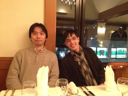
Very brilliant, cool and humble Prof. Kimura |
|
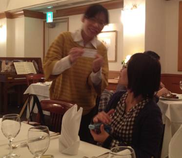
Dr. Ishizaki and Dr. Adachi. I’m impressed with Ishizaki-san’s oyaji gag jokes. Hara-san and I are still thinking whether Adachi-san is really 奥ゆかしい or not. She thinks so though. Lol. Just kidding, Dr. Adachi.
|
|
|
Also the jimu members also treated me nicely and were such a big help in terms of survival. Thanks to Ms. Sakakibara for taking me to the clinic when I caught fever and to Ms. Yuriko Dono for sending me updates on informal seminars inside the facility.
I was able to attend an international workshop on downscaling during my first day as intern. Without even meeting my boss due to personal reasons, I had the opportunity to meet prestigious climatologists in Tsukuba. Also, I joined other informal seminars such as the status of snow in Siberia and I did three presentations. The first one was to introduce my background and plans during the internship. The second was to show some initial findings of the difference between sea surface temperature (SST) datasets. The third was the final presentation which constituted most of my tasks.
|
The first slide of my final presentation |
It is a known fact that SST plays a big role in land-atmosphere circulation. SST may have some impacts to low-lying urban areas as well. We’ve been using almost the same source of SST for our Weather Research and Forecasting (WRF) simulations without evaluating them and knowing how much impact they have in the simulation.
My goal during the internship was to investigate the impacts of various SST datasets as input for WRF-ARW. Three SST datasets (MODIS, NCEP, and OISSTv2) were compared on simulating winter from 2005-2006, and summer of August 2010.
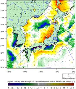
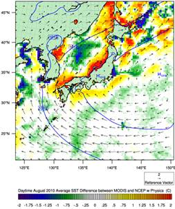
I won’t be discussing the results in detail but it was found that varying only the boundary condition of SST will have some effects to the temperature to as high as 2 km during winter and 1 km during summer. Comparing Moderate Resolution Imaging Spectroradiometer (MODIS) SST (4 km resolution) and National Center for Environmental Prediction (NCEP) SST (1 deg resolution) for example will have differences to as high as 1degC near the coastlines at Aichi prefecture and Hokuriku region during winter and 0.3~degC during summer. Night time also has larger differences compared to daytime. Findings also hint huge differences in the volume of snow simulated during winter when MODIS and Optimum Interpolation Sea Surface Temperature (OISSTv2) were compared. More analyses are currently being conducted. For the meantime, please check out the selected images and animation below. The simulations only differ in terms of SST.
Here shows the WRF simulated monthly average SST differences between MODIS and NCEP for February, 2006 and August, 2010. Difference = MODIS(SST) ? NCEP(SST)
The animation shows the time variation of QCLOUD (Cloud Mixing Ratio) iso-surface (0.0003kg/kg) at 3-hr interval for a selected date on February 2006. Vectors represent wind velocity in m/s.
QCLOUD iso-surface (0.00001kg/kg) at 3-hr interval.
How does the SST indirectly affect the cloud mixing ratios I just showed? Is this really an effect of SST? Well, have a good brain exercise and if you get the answer contact me! ;-)
Note: The images were created using NCAR Command Language (NCL). The animations were made using NCAR’s Visualization and Analysis Platform for Ocean, Atmosphere, and Solar Researchers (VAPOR). The contents are also credited to The Japan Agency for Marine-Earth Science and Technology (JAMSTEC).